Metabolic Phenotyping Protocol Part 3

Implementing the Statistical Analysis in Metabolic Phenotyping Protocol of Blaise et al.

• Part 1 of this series is here.
• Part 2 of this series is here.

If you aren’t familiar with ChemoSpec, you might wish to look at the introductory vignette first.

In this series of posts we are following the protocol as described in the printed publication closely (Blaise et al. 2021). The authors have also provided a Jupyter notebook. This is well worth your time, even if Python is not your preferred language, as there are additional examples and discussion for study.

Read in the Data

Load the Spectra object we created in Part 2 so we can summarize it.

library("ChemoSpec")
load("Worms2.RData")  # restores the 'Worms2' Spectra object
sumSpectra(Worms2)

 C. elegans metabolic phenotyping study (Blaise 2007) 

    There are 133 spectra in this set.
    The y-axis unit is intensity.

    The frequency scale runs from
    8.9995 to 5e-04 ppm
    There are 8600 frequency values.
    The frequency resolution is
    0.001 ppm/point.

    This data set is not continuous
    along the frequency axis.
    Here are the data chunks:

  beg.freq end.freq   size beg.indx end.indx
1   8.9995   5.0005 -3.999        1     4000
2   4.5995   0.0005 -4.599     4001     8600

    The spectra are divided into 4 groups: 

   group no.     color symbol alt.sym
1 Mut_L2  28 #FB0D16FF      0      m2
2 Mut_L4  33 #FFC0CBFF     15      m4
3  WT_L2  32 #511CFCFF      1      w2
4  WT_L4  40 #2E94E9FF     16      w4


*** Note: this is an S3 object
of class 'Spectra'

Exploratory Data Analysis, Con’t.

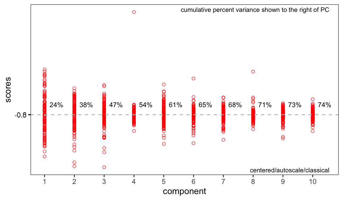
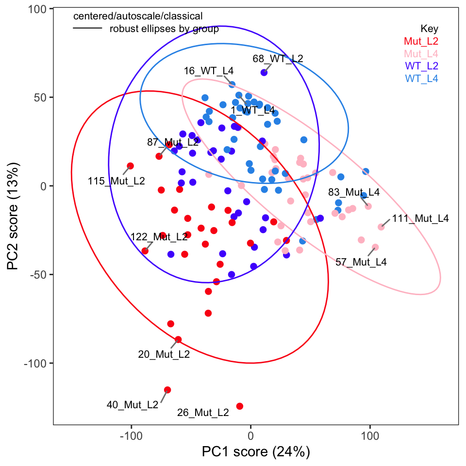
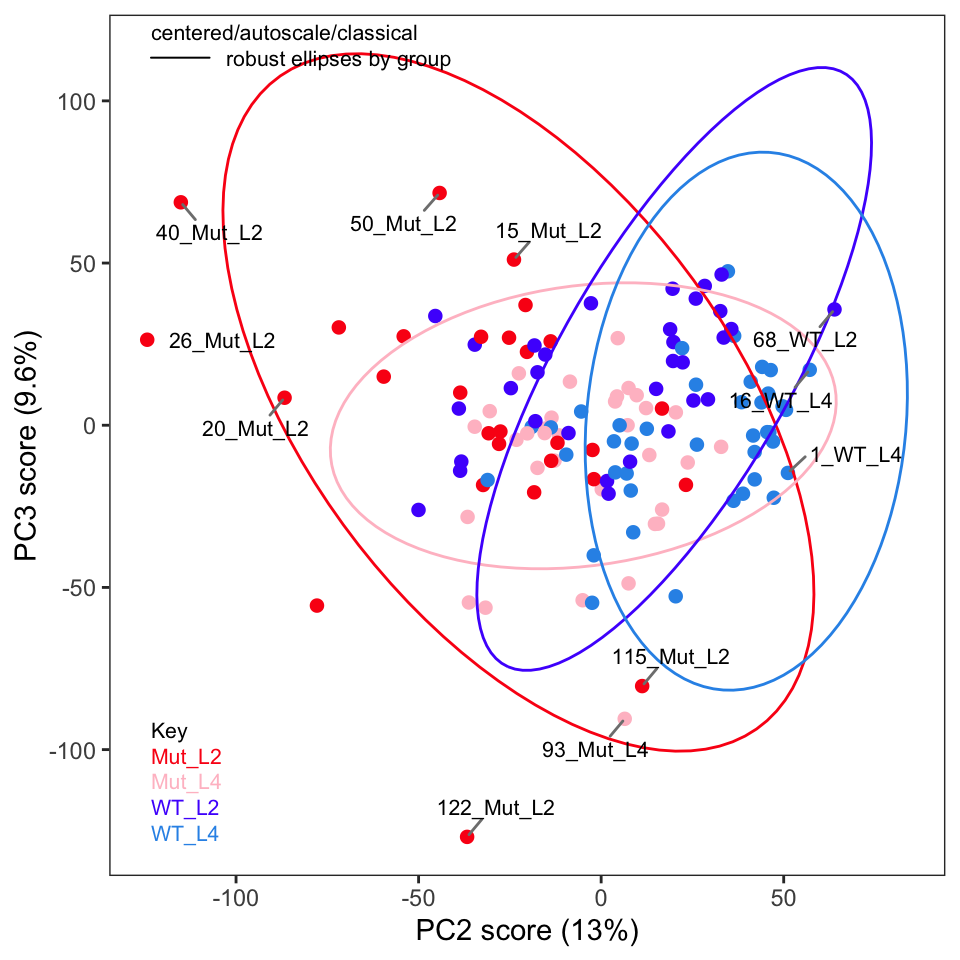
If you recall in Part 2 we removed five samples. Let’s re-run PCA without these samples and show the key plots. We will simply report these here without much discussion; they are pretty much as expected.

c_pca <- c_pcaSpectra(Worms2, choice = "autoscale")

plotScree(c_pca)

Figure 1: Scree plot (recommended style).

p <- plotScores(Worms2, c_pca, pcs = 1:2, ellipse = "rob", tol = 0.02)
p

Figure 2: Score plot for PCs 1 and 2. Compare to protocol figure 7d.

p <- plotScores(Worms2, c_pca, pcs = 2:3, ellipse = "rob", leg.loc = "bottomleft",
    tol = 0.02)
p

Figure 3: Score plot for PCS 2 and 3.

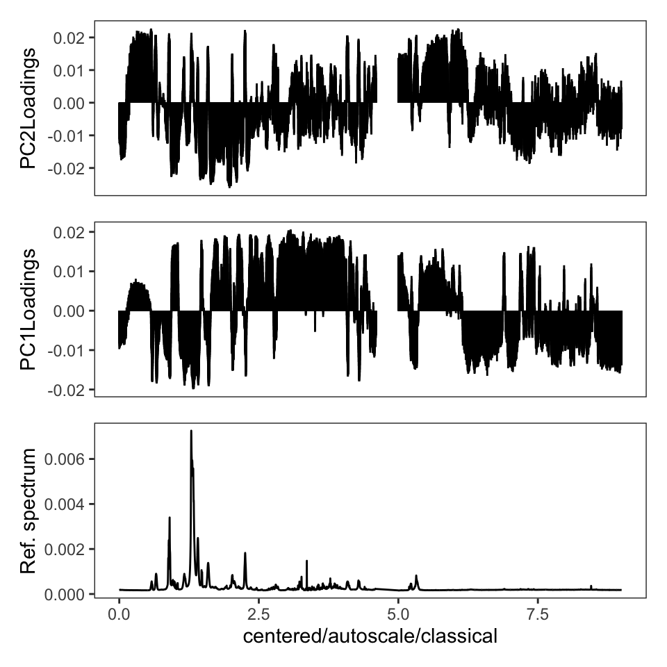
One thing the published protocol does not explicitly discuss is an inspection of the loadings, but it is covered in the Jupyter notebook. The loadings are useful in order to see if any particular frequencies are driving the separation of the samples in the score plot. Let’s plot the loadings (Figure 4). Remember that these data were autoscaled, and hence all frequencies, including noisy frequencies, will contribute to the separation. If we had not scaled the data, these plots would look dramatically different.

p <- plotLoadings(Worms2, c_pca, loads = 1:2)
p

Figure 4: Loadings for PC1 and PC2.

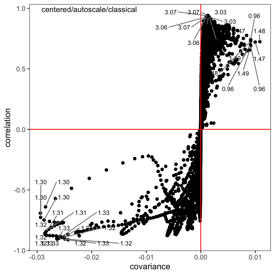
The s-plot is another very useful way to find peaks that are important in separating the samples (Figure 5); we can see that the peaks around \(\delta\) 1.30-1.32, 1.47-1.48, and 3.03-3.07 are important drivers of the separation in the score plot. Having discovered this, one can investigate the source of those peaks.

p <- sPlotSpectra(Worms2, c_pca, tol = 0.001)
p

Figure 5: s-Plot for PC1.

Supervised Analysis with PLS-DA

ChemoSpec carries out exploratory data analysis, which is an unsupervised process. The next step in the protocol is PLS-DA (partial least squares - discriminant analysis). I have written about ChemoSpec + PLS here if you would like more background on plain PLS. However, PLS-DA is a technique that combines data reduction/variable selection along with classification. We’ll need the mixOmics package (F et al. (2017)) package for this analysis; note that loading it replaces the plotLoadings function from ChemoSpec.

library("mixOmics")

Loading required package: MASS

Loading required package: lattice

Loaded mixOmics 6.20.0
Thank you for using mixOmics!
Tutorials: http://mixomics.org
Bookdown vignette: https://mixomicsteam.github.io/Bookdown
Questions, issues: Follow the prompts at http://mixomics.org/contact-us
Cite us:  citation('mixOmics')

Attaching package: 'mixOmics'

The following object is masked from 'package:ChemoSpec':

    plotLoadings

Figure 6 shows the score plot; the results suggest that classification and modeling may be successful. The splsda function carries out a single sparse computation. One computation should not be considered the ideal answer; a better approach is to use cross-validation, for instance the bootsPLS function in the bootsPLS package (Rohart, Le Cao, and Wells (2018) which uses splsda under the hood). However, that computation is too time-consuming to demonstrate here.

X <- Worms2$data
Y <- Worms2$groups
splsda <- splsda(X, Y, ncomp = 8)

plotIndiv(splsda,
  col.per.group = c("#FB0D16FF", "#FFC0CBFF", "#511CFCFF", "#2E94E9FF"),
  title = "sPLS-DA Score Plot", legend = TRUE, ellipse = TRUE)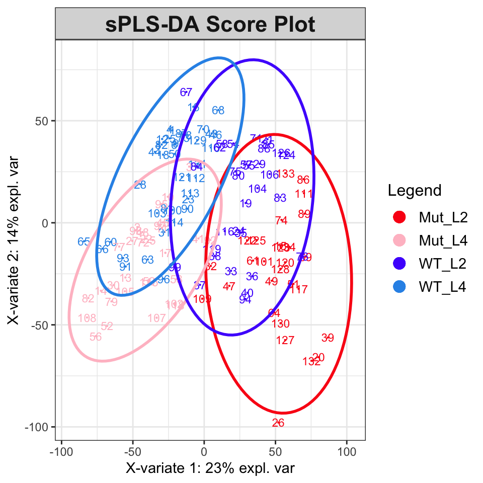

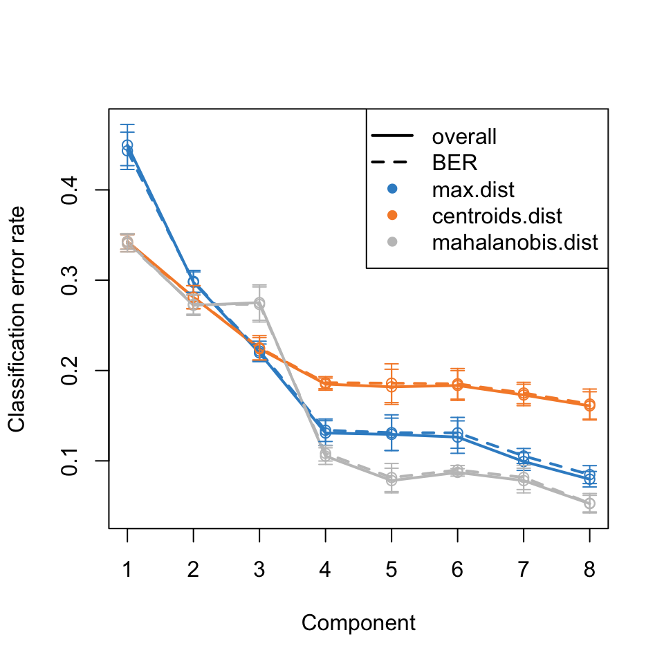
Figure 6: sPLS-DA plot showing classification.

To estimate the number of components needed, the perf function can be used. The results are in Figure 7 and suggest that five components are sufficient to describe the data.

perf.splsda <- perf(splsda, folds = 5, nrepeat = 5)
plot(perf.splsda)

Figure 7: Evaluation of the PLS-DA performance.

At this point, we have several ideas of how to proceed. Going forward, one might choose to focus on accurate classification, or on determining which frequencies should be included in a predictive model. Any model will need to refined and more details extracted. The reader is referred to the case study from the mixOmics folks which covers these tasks and explains the process.

---

This post was created using ChemoSpec version 6.1.3 and ChemoSpecUtils version 1.0.0.

References

Blaise, Benjamin J., Gonçalo D. S. Correia, Gordon A. Haggart, Izabella Surowiec, Caroline Sands, Matthew R. Lewis, Jake T. M. Pearce, et al. 2021. “Statistical Analysis in Metabolic Phenotyping.” Nature Protocols 16: 4299–4326. https://doi.org/10.1038/s41596-021-00579-1.

F, Rohart, Gautier B, Singh A, and Le Cao K-A. 2017. “mixOmics: An r Package for ’Omics Feature Selection and Multiple Data Integration.” PLoS Computational Biology 13 (11): e1005752. http://www.mixOmics.org.

Rohart, Florian, Kim-Anh Le Cao, and Christine Wells. 2018. bootsPLS: Bootstrap Subsamplings of Sparse Partial Least Squares - Discriminant Analysis for Classification and Signature Identification. https://CRAN.R-project.org/package=bootsPLS.