Notes on Linear Algebra Part 2

Motivations - Bushwhacking through the thicket of linear algebra

TL;DR

• Linear algebra is complex. We need a way to penetrate the thicket. Here’s one.
• Linear systems of equations are at the heart, not surprisingly, of linear algebra.
• A key application is linear regression, which has a matrix solution.
• Solving the needed equations requires inverting a matrix.
• Inverting a matrix is more easily done after decomposing the matrix into upper and lower triangular matrices.
• The upper and lower triangular matrices are individually easy to invert, giving access to the inverse of the original matrix.
• Changes in notations and symbols as you move between presentations add significantly to the cognitive burden in learning this material.

---

For Part 1 of this series, see here.

If you open a linear algebra text, it’s quickly apparent how complex the field is. There are so many special types of matrices, so many different decompositions of matrices. Why are all these needed? Should I care about null spaces? What’s really important? What are the threads that tie the different concepts together? As someone who is trying to improve their understanding of the field, especially with regard to its applications in chemometrics, it can be a tough slog.

In this post I’m going to try to demonstrate how some simple chemometric tasks can be solved using linear algebra. Though I cover some math here, the math is secondary right now – the conceptual connections are more important. I’m more interested in finding (and sharing) a path through the thicket of linear algebra. We can return as needed to expand the basic math concepts. The cognitive effort to work through the math details is likely a lot lower if we have a sense of the big picture.

In this post, matrices, including row and column vectors, will be shown in bold e.g. \(\mathbf{A}\) while scalars and variables will be shown in script, e.g. \(n\). Variables used in R code will appear like A.

Systems of Equations

If you’ve had algebra, you have certainly run into “system of equations” such as the following:

\[ \begin{multline} x + 2y -3z = 3 \\ 2x - y - z = 11 \\ 3x + 2y + z = -5 \\ \end{multline} \tag{1}\]

In algebra, such systems can be solved several ways, for instance by isolating one or more variables and substituting, or geometrically (particularly for 2D systems, by plotting the lines and looking for the intersection). Once there are more than a few variables however, the only manageable way to solve them is with matrix operations, or more explicitly, linear algebra. This sort of problem is the core of linear algebra, and the reason the field is called linear algebra.

To solve the system above using linear algebra, we have to write it in the form of matrices and column vectors:

\[ \begin{bmatrix} 1 & 2 & -3 \\ 2 & -1 & -1 \\ 3 & 2 & 1 \\ \end{bmatrix} \begin{bmatrix} x \\ y \\ z \end{bmatrix} = \begin{bmatrix} 3 \\ 11 \\ -5 \end{bmatrix} \tag{2}\]

or more generally

\[ \mathbf{A}\mathbf{x} = \mathbf{b} \tag{3}\]

where \(\mathbf{A}\) is the matrix of coefficients, \(\mathbf{x}\) is the column vector of variable names¹ and \(\mathbf{b}\) is a column vector of constants. Notice that these matrices are conformable:²

\[ \mathbf{A}^{3 \times 3}\mathbf{x}^{3 \times 1} = \mathbf{b}^{3 \times 1} \tag{4}\]

To solve such a system, when we have \(n\) unknowns, we need \(n\) equations.³ This means that \(\mathbf{A}\) has to be a square matrix, and square matrices play a special role in linear algebra. I’m not sure this point is always conveyed clearly when this material is introduced. In fact, it seems like many texts on linear algebra seem to bury the lede.

To find the values of \(\mathbf{x} = x, y, z\)⁴, we can do a little rearranging following the rules of linear algebra and matrix operations. First we pre-multiply both sides by the inverse of \(\mathbf{A}\), which then gives us the identity matrix \(\mathbf{I}\), which drops out.⁵

\[ \mathbf{A}^{-1}\mathbf{A}\mathbf{x} = \mathbf{I}\mathbf{x} = \mathbf{x} = \mathbf{A}^{-1}\mathbf{b} \tag{5}\]

So it’s all sounding pretty simple right? Ha. This is actually where things potentially break down. For this to work, \(\mathbf{A}\) must be invertible, which is not always the case.⁶ If there is no inverse, then the system of equations either has no solution or infinite solutions. So finding the inverse of a matrix, or discovering it doesn’t exist, is essential to solving these systems of linear equations.⁷ More on this eventually, but for now, we know \(\mathbf{A}\) must be a square matrix and we hope it is invertible.

A Key Application: Linear Regression

We learn in algebra that a line takes the form \(y = mx + b\). If one has measurements in the form of \(x, y\) pairs that one expects to fit to a line, we need linear regression. Carrying out a linear regression is arguably one of the most important, and certainly a very common application of the linear systems described above. One can get the values of \(m\) and \(b\) by hand using algebra, but any computer will solve the system using a matrix approach.⁸ Consider this data:

\[ \begin{matrix} x & y \\ 2.1 & 11.8 \\ 0.9 & 7.2 \\ 3.9 & 21.5 \\ 3.2 & 17.2 \\ 5.1 & 26.8 \\ \end{matrix} \tag{6}\]

To express this in a matrix form, we recast

\[ y = mx + b \tag{7}\]

into

\[ \mathbf{y} = \mathbf{X}\mathbf{\beta} + \mathbf{\epsilon} \tag{8}\]

where:

• \(\mathbf{y}\) is the column vector of \(y\) values. That seems sensible.
• \(\mathbf{X}\) is a matrix composed of a column of ones plus a column of the \(x\) values. This is called a design matrix. At least here \(\mathbf{X}\) contains only \(x\) values as variables.
• \(\mathbf{\beta}\) is a column vector of coefficients (including, as we will see, the values of \(m\) and \(b\) if we are thinking back \(y = mx + b\)).
• \(\mathbf{\epsilon}\) is new, it is a column vector giving the errors at each point.

With our data above, this looks like:

\[ \begin{bmatrix} 11.8 \\ 7.2 \\ 21.5 \\ 17.2 \\ 26.8 \\ \end{bmatrix} = \begin{bmatrix} 1 & 2.1 \\ 1 & 0.9 \\ 1 & 3.9 \\ 1 & 3.2 \\ 1 & 5.1 \\ \end{bmatrix} \begin{bmatrix} \beta_0 \\ \beta_1 \end{bmatrix} + \begin{bmatrix} \epsilon_1 \\ \epsilon_2 \\ \epsilon_3 \\ \epsilon_4 \\ \epsilon_5 \end{bmatrix} \tag{9}\]

If we multiply this out, each row works out to be an instance of \(y_i = \beta_1 x_i + \beta_0\). Hopefully you can appreciate that \(\beta_1\) corresponds to \(m\) and \(\beta_0\) corresponds to \(b\).⁹

This looks similar to \(\mathbf{A}\mathbf{x} = \mathbf{b}\) seen in Equation 3, if you set \(\mathbf{b}\) to \(\mathbf{y}\), \(\mathbf{A}\) to \(\mathbf{X}\) and \(\mathbf{x}\) to \(\beta\):

\[ \begin{align} \mathbf{b} &\approx \mathbf{A}\mathbf{x} \\ \downarrow &\phantom{\approx} \; \downarrow \; \downarrow \\ \mathbf{y} &\approx \mathbf{X}\mathbf{\beta} \\ \end{align} \tag{10}\]

This contortion of symbols is pretty nasty, but honestly not uncommon when moving about in the world of linear algebra.

As it is composed of real data, presumably with measurement errors, there is not an exact solution to \(\mathbf{A}\mathbf{x} = \mathbf{b}\) due to the error term. There is however, an approximate solution, which is what is meant when we say we are looking for the line of best fit. This is how linear regression is carried out on a computer. The relevant equation is:

\[ \hat{\beta} = (\mathbf{X}^{\mathsf{T}}\mathbf{X})^{-1}\mathbf{X}^{\mathsf{T}}y \tag{11}\]

The key point here is that once again we need to invert a matrix to solve this. The details of where Equation 11 comes from are covered in a number of places, but I will note here that \(\hat{\beta}\) refers to the best estimate of \(\beta\).¹⁰

Inverting Matrices

We now have two examples where inverting a matrix is a key step: solving a system of linear equations, and approximating the solution to a system of linear equations (the regression case). These cases are not outliers, the ability to invert a matrix is very important. So how do we do this? The LU decomposition can do it, and is widely used so worth spending some time on. A decomposition is the process of breaking a matrix into pieces that are easier to handle, or that give us special insight, or both. If you are a chemometrician you have almost certainly carried out Principal Components Analysis (PCA). Under the hood, PCA requires either a singular value decomposition, or an eigen decomposition (more info here).

So, about the LU decomposition: it breaks a matrix into two matrices, \(\mathbf{L}\), a “lower triangular matrix”, and \(\mathbf{U}\), an “upper triangular matrix”. These special matrices contain only zeros except along the diagonal and the entries below it (in the lower case), or along the diagonal and the entries above it (in the upper case). The advantage of triangular matrices is that they are very easy to invert (all those zeros make many terms drop out). So the LU decomposition breaks the tough job of inverting \(\mathbf{A}\) into two easier jobs.

\[ \begin{align} \mathbf{A} &= \mathbf{L}\mathbf{U} \\ \mathbf{A}^{-1} &= (\mathbf{L}\mathbf{U})^{-1} \\ \mathbf{A}^{-1} &= \mathbf{U}^{-1}\mathbf{L}^{-1} \\ \end{align} \tag{12}\]

When all is done, we only need to figure out \(\mathbf{U}^{-1}\) and \(\mathbf{L}^{-1}\) which as mentioned is straightforward.¹¹

To summarize, if we want to solve a system of equations we need to carry out matrix inversion, which is turn is much easier to do if one uses the LU decomposition to get two easy to invert triangular matrices. I hope you are beginning to see how pieces of linear algebra fit together, and why it might be good to learn more.

R Functions

Inverting Matrices

Let’s look at how R does these operations, and check our understanding along the way. R makes this really easy. We’ll start with the issue of invertibility. Let’s create a matrix for testing.

A1 <- matrix(c(3, 5, -1, 11, 2, 0, -5, 2, 5), ncol = 3)
A1

     [,1] [,2] [,3]
[1,]    3   11   -5
[2,]    5    2    2
[3,]   -1    0    5

In the matlib package there is a function inv that inverts matrices. It returns the inverted matrix, which we can verify by multiplying the inverted matrix by the original matrix to give the identity matrix (if inversion was successful). diag(3) creates a 3 x 3 matrix with 1’s on the diagonal, in other words an identity matrix.

library("matlib")
A1_inv <- inv(A1)
all.equal(A1_inv %*% A1, diag(3)) 

[1] "Mean relative difference: 8.999999e-08"

The difference here is really small, but not zero. Let’s use a different function, solve which is part of base R. If solve is given a single matrix, it returns the inverse of that matrix.

A1_solve <- solve(A1) %*% A1
all.equal(A1_solve, diag(3))

[1] TRUE

That’s a better result. Why are there differences? inv uses a method called Gaussian elimination which is similar to how one would invert a matrix using pencil and paper. On the other hand, solve uses the LU decomposition discussed earlier, and no matrix inversion is necessary. Looks like the LU decomposition gives a somewhat better numerical result.

Now let’s look at a different matrix, created by replacing the third column of A1 with different values.

A2 <- matrix(c(3, 5, -1, 11, 2, 0, 6, 10, -2), ncol = 3)
A2

     [,1] [,2] [,3]
[1,]    3   11    6
[2,]    5    2   10
[3,]   -1    0   -2

And let’s compute its inverse using solve.

solve(A2)

Error in solve.default(A2): system is computationally singular: reciprocal condition number = 6.71337e-19

When R reports that A2 is computationally singular, it is saying that it cannot be inverted. Why not? If you look at A2, notice that column 3 is a multiple of column 1. Anytime one column is a multiple of another, or one row is a multiple of another, then the matrix cannot be inverted because the rows or columns are not independent.¹² If this was a matrix of coefficients from an experimental measurement of variables, this would mean that some of your variables are not independent, they must be measuring the same underlying phenomenon.

Solving Systems of Linear Equations

Let’s solve the system from Equation 2. It turns out that the solve function also handles this case, if you give it two arguments. Remember, solve is using the LU decomposition behind the scenes, no matrix inversion is required.

A3 <- matrix(c(1, 2, 3, 2, -1, 2, -3, -1, 1), ncol = 3)
A3

     [,1] [,2] [,3]
[1,]    1    2   -3
[2,]    2   -1   -1
[3,]    3    2    1

colnames(A3) <-c("x", "y", "z") # naming the columns will label the answer
b <- c(3, 11, -5)
solve(A3, b)

 x  y  z 
 2 -4 -3 

The answer is the values of \(x, y, z\) that make the system of equations true.

How does LU decomposition avoid inversion?

While we’ve emphasized the importance and challenges of inverting matrices, we’ve also pointed out that to solve a linear system there are alternatives to looking at the problem from the perspective of Equation 5. Here’s an approach using the LU decomposition, starting with substituting \(\mathbf{A}\) with \(\mathbf{L}\mathbf{U}\):

\[ \mathbf{A}\mathbf{x} = \mathbf{L}\mathbf{U}\mathbf{x} = \mathbf{b} \tag{13}\]

We want to solve for \(\mathbf{x}\) the column vector of variables. To do so, define a new vector \(\mathbf{y} = \mathbf{U}\mathbf{x}\) and substitute it in:

\[ \mathbf{L}\mathbf{U}\mathbf{x} = \mathbf{L}\mathbf{y} = \mathbf{b} \tag{14}\]

Next we solve for \(\mathbf{y}\). One way we could do this is to pre-multiply both sides by \(\mathbf{L}^{-1}\) but we are looking for a way to avoid using the inverse. Instead, we evaluate \(\mathbf{L}\mathbf{y}\) to give a series of expressions using the dot product (in other words plain matrix multiplication). Because \(\mathbf{L}\) is lower triangular, many of the terms we might have gotten actually disappear because of the zero coefficients. What remains is simple enough that we can algebraically find each element of \(\mathbf{y}\) starting from the first row (this is called forward substitution). Once we have \(\mathbf{y}\), we can find \(\mathbf{x}\) by solving \(\mathbf{y} = \mathbf{U}\mathbf{x}\) using a similar approach, but working from the last row upward (this is backward substitution). This is a good illustration of the utility of triangular matrices: some operations can move from the linear algebra realm to the algebra realm. Wikipedia has a good illustration of forward and backward substitution.

Computing Linear Regression

Let’s compute the values for \(m, b\) in our regression data shown in Equation 6. First, let’s set up the needed matrices and plot the data since visualizing the data is always a good idea.

y = matrix(c(11.8, 7.2, 21.5, 17.2, 26.8), ncol = 1)
X = matrix(c(rep(1, 5), 2.1, 0.9, 3.9, 3.2, 5.1), ncol = 2) # design matrix
X

     [,1] [,2]
[1,]    1  2.1
[2,]    1  0.9
[3,]    1  3.9
[4,]    1  3.2
[5,]    1  5.1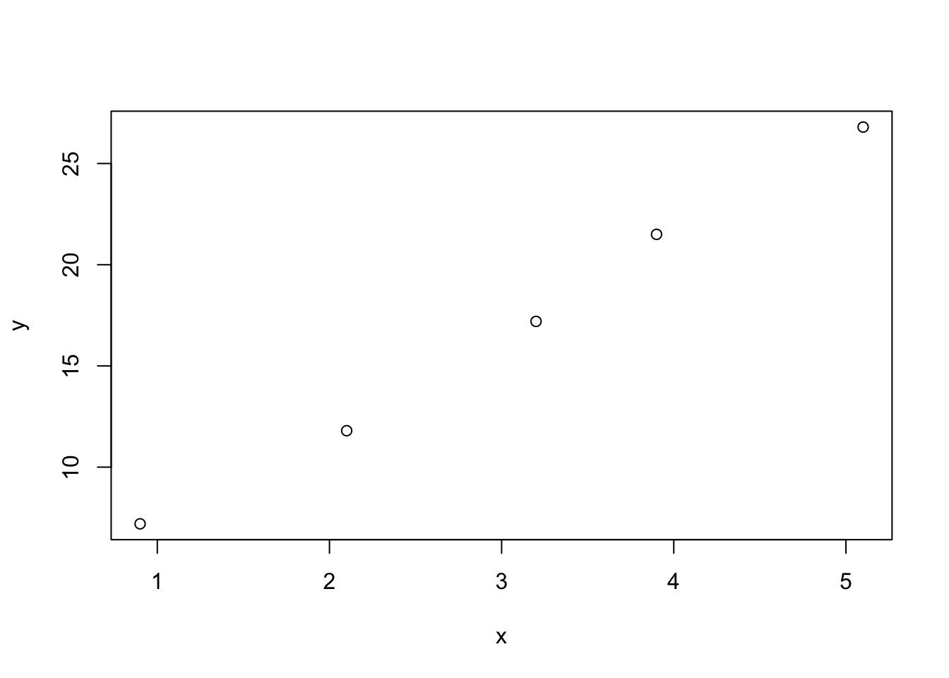

plot(X[,2], y, xlab = "x") # column 2 of X has the x values

The value of \(\hat{\beta}\) can be found via Equation 11:

solve((t(X) %*% X)) %*%  t(X) %*% y

         [,1]
[1,] 2.399618
[2,] 4.769862

The first value is for \(b\) or \(\beta_0\) or intecept, the second value is for \(m\) or \(\beta_1\) or slope.

Let’s compare this answer to R’s built-in lm function (for linear model):

fit <- lm(y ~ X[,2])
fit

Call:
lm(formula = y ~ X[, 2])

Coefficients:
(Intercept)       X[, 2]  
       2.40         4.77  

We have good agreement! If you care to learn about the goodness of the fit, the residuals etc, then you can look at the help file ?lm and str(fit). lm returns pretty much all one needs to know about the results, but if you wish to calculate all the interesting values yourself you can do so by manipulating Equation 11 and its relatives.

Finally, let’s plot the line of best fit found by lm to make sure everything looks reasonable.

plot(X[,2], y, xlab = "x")
abline(coef = coef(fit), col = "red")

---

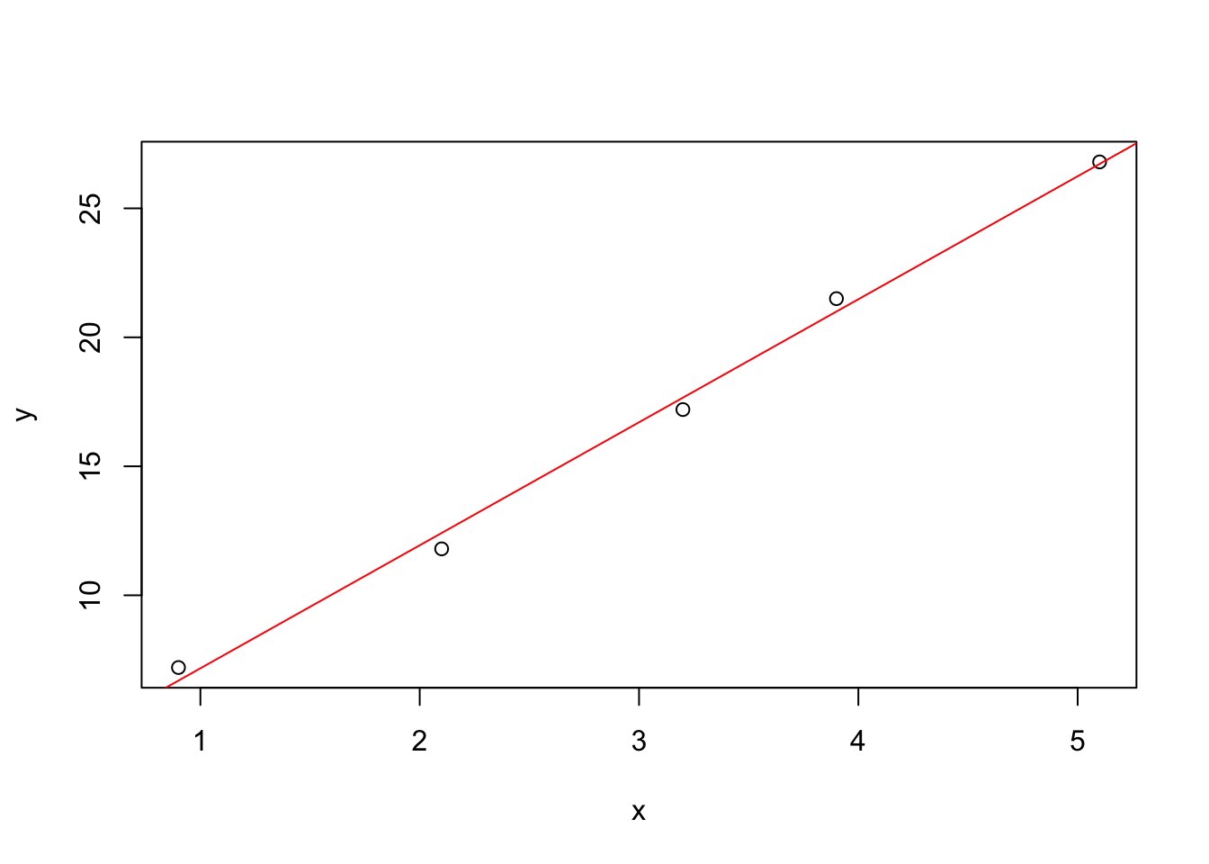
That’s all for now, and a lot to digest. I hope you are closer to finding your own path through linear algebra. Remember that investing in learning the fundamentals prepares you for tackling the more complex topics. Thanks for reading!

Annotated Bibliography

These are the main sources I relied on for this post.

• The No Bullshit Guide to Linear Algebra by Ivan Savov.
  • Section 1.15: Solving systems of linear equations.
  • Section 6.6: LU decomposition.
• Linear Algebra: step by step by Kuldeep Singh, Oxford Univerity Press, 2014.
  • Section 1.8.5: Singluar (non-invertible) matrices mean there is no solution or infinite solutions to the linear system. For graphical illustration see sections 1.1.3 and 1.7.2.
  • Section 1.6.4: Definition of the inverse and conceptual meaning.
  • Section 1.8.4: Solving linear systems when \(\mathbf{A}\) is invertible.
  • Section 6.4: LU decomposition.
  • Section 6.4.3: Solving linear systems without using inversion, via the LU decomposition.
• Linear Models with R by Julian J. Faraway, Chapman and Hall/CRC, 2005.
  • Sections 2.1-2.4: Linear regression from the algebraic and matrix perspectives, derivation of Equation 11.
• The vignettes of the matlib package are very helpful.

Footnotes

1. Here we have the slightly unfortunate circumstance where symbol conventions cannot be completely harmonized. We are saying that \(\mathbf{x} = x, y, z\) which seems a bit silly since vector \(\mathbf{x}\) contains \(y\) and \(z\) components in addition to \(x\). I ask you to accept this for two reasons: First, most linear algebra texts use the symbols in Equation 3 as the general form for this topic, so if you go to study this further that’s what you’ll find. Second, I feel like using \(x\), \(y\) and \(z\) in Equation 1 will be familar to the most people. If you want to get rid of this infelicity, then you have to write Equation 1 (in part) as \(x_1 + 2x_2 + 3x_3 = 3\) which I think clouds the interpretation. Perhaps however you feel my choices are equally bad.

2. Conformable means that the number of columns in the first matrix equals the number of rows in the second matrix. This is necessary because of the dot product definition of matrix multiplication. More details here.

3. Remember “story problems” where you had to read closely to express what was given in terms of equations, and find enough equations? “If Sally bought 10 pieces of candy and a drink for $1.50…”

4. We could also write this as \(\mathbf{x} = (x, y, z)^\mathsf{T}\) to emphasize that it is a column vector. One might prefer this because the only vector one can write in a row of text is a row vector, so if we mean a column vector many people would prefer to write it transposed.

5. The inverse of a matrix is analogous to dividing a variable by itself, since it leads to that variable canceling out and thus simplifying the equation. However, strictly speaking there is no operation that qualifies as division in the matrix world.

6. For a matrix \(\mathbf{A}\) to be invertible, there must exist another matrix \(\mathbf{B}\) such that \(\mathbf{A}\mathbf{B} = \mathbf{B}\mathbf{A} = \mathbf{I}\). However, this definition doesn’t offer any clues about how we might find the inverse.

7. In truth, there are other ways to solve \(\mathbf{A}\mathbf{x} = \mathbf{b}\) that don’t require inversion of a matrix. However, if a matrix \(\mathbf{A}\) isn’t invertible, these other methods will also break down. We’ll demonstrate this later when we talk about the LU decomposition.

8. A very good discussion of the algebraic approach is available here.

9. This is another example of an infelicity of symbol conventions. The typical math/statistics text symbols are not the same as the symbols a student in Physics 101 would likely encounter.

10. The careful reader will note that the data set shown in Equation 9 is not square, there are more observations (rows) than variables (columns). This is fine and desireable for a linear regression, we don’t want to use just two data points as that would have no error but not necessarily be accurate. However, only square matrices have inverses, so what’s going on here? In practice, what’s happening is we are using something called a pseudoinverse. The first part of the right side of Equation 11 is in fact the pseudoinverse: \((\mathbf{X}^{\mathsf{T}}\mathbf{X})^{-1}\mathbf{X}^{\mathsf{T}}\). Perhaps we’ll cover this in a future post.

11. The switch in the order of matrices on the last line of Equation 12 is one of the properties of the inverse operator.

12. This means that the rank of the matrix is less than the number of columns. You can get the rank of a matrix by counting the number of non-zero eigenvalues via eigen(A2)$values, which in this case gives 8.9330344, -5.9330344, -3.5953271^{-16}. There are only two non-zero values, so the rank is two. Perhaps in another post we’ll discuss this in more detail.