Earth’s Field NMR
NMR
EF-NMR
What can we measure? Why or Why Not? Pros? Cons?
TL;DR
- In EF-NMR the line widths are extremely narrow but there is no chemical shift dispersion.
- We can observe heteronuclear couplings in EF-NMR as they are field-invariant.
- In EF-NMR the population of the two energy states is essentially equal, eliminating any signal. We can get around this with pre-polarization.
- The resonance frequency of \(\ce{^{1}H}\) NMR in EF is in the audio range, greatly simplifying the electronics.
Let’s take a closer look from first principles what kinds of information one can glean from EF-NMR. We’ll restrict our discussion to spin \(\frac{1}{2}\) nuclei with ~100% abundance, like \(\ce{^{1}H}\), \(\ce{^{31}P}\) or \(\ce{^{19}F}\) – you’ll see why soon enough. Table 1 gives some relevant physical parameters for these nuclei.
| Nuclei | Gyromagnetic ratio \(\gamma\) | Larmor Freq. |
|---|---|---|
| \(\ce{^{1}H}\) | 26.7522 | 100 |
| \(\ce{^{19}F}\) | 25.1815 | 94 |
| \(\ce{^{31}P}\) | 10.8394 | 40.5 |
Excellent general references on NMR theory are Friebolin (Friebolin 2011) and Claridge (Claridge 2016).
Line Widths are Very Narrow
The line width of an NMR signal is primarily dependent on the homogeneity of the \(B_o\) field, which in the case of earth’s field is very good. Appelt et al. (2006) state that when observations are made >100 meters from buildings and ferrous structures1 the homogeneity of the earth’s magnetic field for small sample volumes is in the range of \(\Delta B/B < 10^{-6}\). They further state that when \(T_1 \sim T_2 > 3\) seconds line widths will be less than 0.1 Hz.2 This all sounds very promising: narrow lines imply good separation between peaks.
No Chemical Shift Information
One of the characteristics of high-field NMR which makes it so useful is the dispersion of chemical shifts as a function of structure. Unfortunately, EF-NMR has effectively zero chemical shift dispersion. The equation for computing chemical shift, \(\delta\), is:
\[ \delta = \frac{\nu_{sample} - \nu_{reference}}{\nu_{B_o}} \]
where the units are:
\[ ppm = \frac{Hz}{MHz} \]
since \(\delta\) is a field strength independent quantity. Taking \(\nu_{reference}\) to be zero, e.g. TMS added to the sample, we can rearrange the equation to get \(\nu_{sample}\). Consider the compound \(\ce{CH3Br}\) whose methyl group has a chemical shift of 2.63 ppm. Using an earth’s field \(\ce{^{1}H}\) Larmor frequency of 19.1 KHz, we can compute the shift of \(\ce{CH3Br}\) in Hz as 0.0191 Hz. This is an extremely small value, smaller than the typical line width in earth’s field (so the promise of narrow line widths is not going to save us).
For further comparison, we can do the same calculation for \(\ce{CH2Br2}\) which has a shift of 4.90 ppm. The result is exactly the same, 0.0191 Hz. We can see that these two compounds with differing numbers of halogens, which would be trivial to distinguish with a low field bench-top instrument operating at 80 MHz, are indistinguishable in earth’s field. This is due to the very small value of earth’s magnetic field.
Heteronuclear Couplings
While the chemical shift dispersion in earth’s field is clearly nil, heteronuclear J couplings are readily observed due to their greater magnitude, up to about 200 Hz. Appelt et al. (2006) gives a number of interesting examples involving \(\ce{^{1}H}\), \(\ce{^{19}F}\) and \(\ce{^{29}Si}\) containing compounds.
Populations of Quantum States
Basic NMR theory tells us that the energy difference between the two quantum states for a spin \(\frac{1}{2}\) nucleus is proportional to the field strength \(B_o\):
\[ \Delta E = \gamma \hbar B_o \]
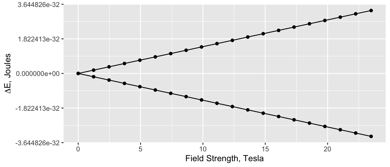
where \(\hbar\) is \(\frac{h}{2\pi}\). A plot for \(\ce{^{1}H}\) is shown in Figure 1; the right-most point corresponds to a 1,000 MHz instrument. Clearly as \(B_o\) goes to zero the \(\Delta E\) goes to zero in a simple linear fashion.
We can then relate the number of nuclei in the upper energy state, \(N_{\beta}\), to that in the lower energy state, \(N_{\alpha}\), at thermal equilibrium as:
\[ \frac{N_{\beta}}{N_{\alpha}} = e^{- \Delta E/kT} \approx 1 - \frac{\Delta E}{kT} = 1- \frac{\gamma \hbar B_o}{kT} \]
where \(k\) is the Boltzman constant and \(T\) is the temperature in Kelvin. The ratio of population states is nearly equal for any value of \(B_o\) but of course gets even worse as \(B_o\) decreases. This is the reason for the low overall sensitivity of NMR as an analytical technique. We can compute the ratio for \(\ce{^{1}H}\) at room temperature; we’ll compare the value for earth’s field to those of a 100 and 1,000 MHz instruments:
      45 uT (Earth)    2.35 T (100 MHz) 23.49 T (1,000 MHz)
     1.000000000000      0.999999999998      0.999999999982
As you can see, in earth’s field there is basically no difference in the two population states, meaning there is no signal to observe. Clearly a problem!
If all the nuclei were in \(N_{\alpha}\) we could measure the energy required to bump them up to \(N_{\beta}\), or more commonly, bump them up and then watch the energy given off as equilibrium returns. Unfortunately, the signal produced is proportional to \(N_{\alpha} - N_{\beta}\), which is effectively zero in earth’s field. At the same time however, the more spins we have, the higher the signal will be. More spins total in the detection coil sweet spot will be helpful, but there are other factors mitigating against making large coils to accommodate large samples. One way around this is to use signal averaging.
Pre-Polarization
In the case of earth’s field NMR, the usual way around this problem of very limited signal is to pre-polarize the sample.3 This basically involves subjecting the sample to a fairly high magnetic field for a brief period before measuring the any signals. This pre-polarization field forces more of the \(N_{\beta}\) nuclei to assume the lower energy \(N_{\alpha}\) state, thus increasing \(N_{\alpha} - N_{\beta}\) which means there is a signal to be observed. Mohorič has an excellent but technical discussion of the details of this process (Mohorič and Stepišnick 2009).
EF-NMR Signals are in the Audio Range
What is the Larmor (resonance) frequency in earth’s field? Earth’s magnetic field varies from about 25 to 65 \(\mu\)T; we’ll use an intermediate value of 45 \(\mu\)T for our calculations. The Larmor frequency is given by the equation:
\[ \nu_{L} = \lvert\frac{\gamma}{2\pi}\rvert B_o \]
Notice there is a simple linear relation between \(\nu_{L}\) and \(B_o\).4 If we plug in values for our nuclei we get the following values in Hz:
       1H       19F       31P
19159.852 18034.921  7763.148
What we have shown here is that for EF-NMR, resonance frequencies are in the audio (20 - 20,000 Hz) and lower radio (20,000 Hz +) frequency range. Why is this important? It greatly simplifies signal detection because audio receivers are essentially radios, and the electronics for working in this frequency range are extremely well worked out, and not expensive to buy or build.
Historical Note
The first earth’s field NMR experiment was apparently conducted by Martin Packard and Russell Varian while at Varian Associates (Packard and Varian 1954). Varian Associates was of course a major instrument player, including NMR, and for a long time marketed their instruments largely toward colleges. 5
References
Appelt, Stephan, Holger Kühn, F. Wolfgang Häsing, and Bernhard Blümich. 2006. “Chemical Analysis by Ultrahigh-Resolution Nuclear Magnetic Resonance in the Earth’s Magnetic Field.” Nature Physics 2. https://doi.org/10.1038/nphys211.
Claridge, Timothy D. W. 2016. High-Resolution NMR Techniques in Organic Chemistry. Elsevier.
Friebolin, Horst. 2011. Basic One- and Two-Dimensional NMR Spectroscopy. Wiley-VCH.
Mohorič, Aleš, and Janez Stepišnick. 2009. “NMR in the Earth’s Magnetic Field.” Progress in Nuclear Magnetic Resonance Spectroscopy 54: 166–82. https://doi.org/10.1016/j.pnmrs.2008.07.002.
Packard, Martin, and Russell Varian. 1954. “Free Nuclear Induction in the Earth’s Magnetic Field.” Physical Review 93: 939.
Footnotes
Keep in mind that buried utilities made of iron or carrying electrical current can interfere.↩︎
\(T_1\) is the relaxation time for magnetization aligned with the \(B_o\) axis, which corresponds to the \(z\) axis. This is the relaxation time that affects the ability to pulse quickly. It’s also called the spin-lattice relaxation time. \(T_2\) is the relaxation time corresponding to magnetization in the \(x,y\) plane, and is also known as the spin-spin relaxation time. \(T_2\) is largely determined by magnetic field inhomogeneity and the line width at half peak height is \(\Delta \nu_{1/2} = \gamma \Delta B_o /2\). \(T_1 \ge T_2\). See Friebolin chapter 7 for a detailed discussion.↩︎
In fact pre-polarizing or polarizing the sample is now en-vogue for higher field instruments as well, in the form of DNP, SABRE etc.↩︎
The gyromagnetic ratio can be negative, hence the absolute value is taken here.↩︎
Martin Packard is apparently unrelated to David Packard, one of the founders of HP.↩︎
Reuse
Citation
BibTeX citation:
@online{hanson2023,
  author = {Hanson, Bryan},
  title = {Earth’s {Field} {NMR}},
  date = {2023-07-26},
  url = {http://chemospec.org/posts/2023-07-19-EF-NMR-1/EF-NMR-1.html},
  langid = {en}
}
For attribution, please cite this work as:
Hanson, Bryan. 2023. “Earth’s Field NMR.” July 26, 2023. http://chemospec.org/posts/2023-07-19-EF-NMR-1/EF-NMR-1.html.